MPS Rx
 The detected particle signal is always superimposed by some amount of drive field feedthrough, and to minimize this, we use a gradiometric receive coil. While there have been a few proposed designs (all which have pros and cons and discussed further below) we have elected to use a two-part gradiometer of 50 turns per side (100 total). The gradiometer has a resistance of 1.9 Ohms (@23.8 kHz) and an inductance of 31 uH.
The parameters of this coil are chosen based on a few assumptions: The length of each coil (receive and cancellation part) should be bigger than its radius to maximize the homogeneity of the sensitive region. A certain distance between both coils is also needed to prevent signal in one coil from significantly inducing a signal in the opposite one. Both coils should also be located in the homogeneous part of the drive field to detect the same field and enable more accurate Tx decoupling.
To get a high induced voltage through the particles, a high turn density is necessary. To reach that, we are using an in-house made Litz wire consisting of 5 stands of parallel thin magnet wire (28/5 AWG Litz, which is 5 strands of ~0.3mm diameter) and determined the number of turns to roughly have the length of wire equal the length of wire on the Tx coil. This turn count (50 each half) is roughly appropriate anyway to balance coil noise, Rx coil inductance, and parasitic capacitance.
As mentioned, there are many different designs for "gradiometers", but first it is worth defining what a "gradiometer" is and why it is called that. As the name implies, the gradiometer measures the magnetic gradient/differential induced due to particles disrupting the otherwise homogeneous drive field. Now, this principle can be manifested in many forms--below are three illustrations of designs that have been used. In each design, the functional principle is the same, with the goal to be to minimize the baseline signal due to the drive field.
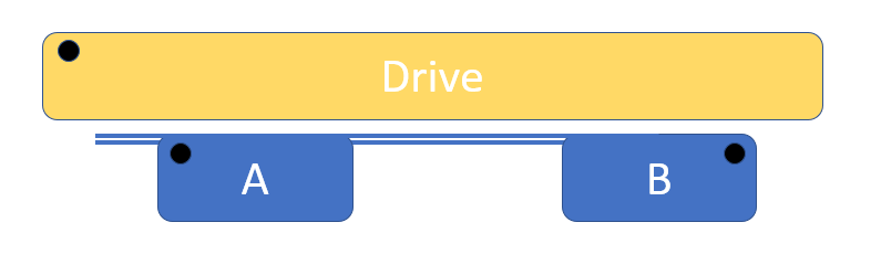
Design A: The design currently employed in the MPS system, with the difference that the drive is not a single solenoid, but the fields are effectively the same.
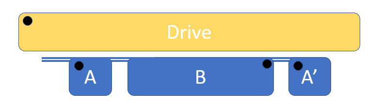
Design B: A gradiometer design discussed in many papers, one notable example being this paper by M. Graeser et al. [1].
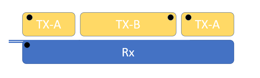
Design C: A gradiometric drive coil arrangement presented in this paper [2]
In these designs, there are pros and cons associated with each. Here are my personal thoughts on each of these selected designs and why we elected for the top one (design A)
A: Pros: Simple to implement, easy to adjust mechanically, robust design Cons: Low efficiency because the sensitive regions (coils A/B) are near the edges of the drive/ bias field they need to be longer to create the required fields within the Rx coils (i.e. the drive/bias field is strongest in the center of the coil, yet there is no receive coil there so that energy is wasted.
B: Pros: More efficient because the strongest field (bias/drive) is at the center where the Rx coil with particles are. Cons: A bit more mechanically complex to adjust and implement-- despite this, other groups have had success and high feedthrough attenuation
C: Pros: very simple Rx coil and it can probably have a very narrow diameter allowing for a more narrow Tx coil which would then improve efficiency by limiting edge effects. It also allows for the possibility to electrically tune the gradiometer by differentially powering the two drive coils (though I haven't seen this implemented in literature yet, and sounds challenging to do reliably). Cons: There may be destructive interference of the Tx coils lowering efficiency depending on the exact geometry.
We went with design A because of its reliable and simple nature.
As stated above, we are currently using a 100 turn Rx coil (50 per side of the gradiometer) with results in both a fairly low resistance (~2 Ohms) and moderate inductance (~30uH)
One issue with adding more turns to get more signal is that the real resistive load is that it manifests both in more thermal voltage noise, it increases the voltage stemming from current noise in the amplifier (a helpful discussion here from Analog Device)
The other issue with adding more turns is it increases the inductance, which increases the effect of current noise and reduction of bandwidth. The Bandwith issue associated with high inductances stems from the inductors' inherent property of increasing impedance with frequency, and thus acting as a low-pass filter with the input impedance of the amplifier (or its own parasitic capacitance). For magnetometry and relaxometry where the primary signal is in the lower harmonics, this is less of an issue, especially when driving at 10-25kHz. But for spectroscopy when the primary goal is to see the harmonic distortion created by the nonlinearity in the particles' magnetization, this limitation can be profound.
To make the wire, 5 strands of 28AWG wire was measured and cut to about 25% longer than the calculated necessary length. One end of these wires was fixed around a stationary post, and the other ends were tied together to form a loop. This loop was put into a drill and the bundle of wires were twisted while maintaining light tension. This resulting bundle of wire was wound around the Rx coil former (glass tube). Each wire's insulation was stripped ~1cm from the end, fluxed, twisted, and then soldered together. After winding, the two wires were attached to a shielded twisted pair, where the two twisted wires were the signals, and the shield was attached to ground (grounded on one end only!).
 [1] M. Graeser et al. Towards Picogram Detection of Superparamagnetic Iron-Oxide Particles Using a Gradiometric Receive Coil
 [2] D. Pantke et al. Multifrequency magnetic particle imaging enabled by a combined passive and active drive field feed‐through compensation approach